Building SQL Project With E-Commerce Dataset From Kaggle
Sales analysis is used to determine how well some products are selling by comparing their sales target with the actual sales. It also helps us to discover insights such as popular and underperforming products, market trends, high-value customers, etc. In this article, I will explain how I performed sales analysis on the dataset containing sales details from an Indian e-commerce website. This e-commerce dataset was obtained from Kaggle.🧐
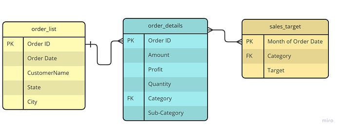
For your information, I performed the analysis using MySQL workbench. I have created a PDF showing the steps to create a new schema and import datasets to the MySQL workbench. You may refer to this PDF if you are not sure how to perform these steps. Below is the entity-relationship diagram that I created with the help of a template on MIRO.

Before performing the analysis, I used the following commands to rename the columns which contain space or dash in their names.

Below are the hypothetical questions I created on my own, my solutions, and the results. 🤓
Query 1: The marketing department is running a sales campaign and they target the customer with different sales materials. They categorized customers into groups based on the RFM model. Show the number and percentage for each customer segment as the final result. Order the results by the percentage of customers.

For the sake of convenience, a view called “combined_orders” was created by joining the “order_details” and “order_list”. Another view called “customer_grouping” was created by using a subquery (aka nested query).
In the inner query, I used the STR_TO_DATE() function is used to convert “order_date” from string to date format. To find the recency for each customer, I used DATEDIFF() function to find the difference between the 31st of March 2019 (the final date in the dataset) and the latest transaction date for each customer.
The NTILE() function is used to separate the customers into groups based on the recency, frequency, and monetary of the customers. We rank these customers from 1–5 using RFM values. Since we do not favor long customer inactivity and this function starts from 1, we order the recency in descending order, so that the inactive customers would be given lower recency. We prefer customers to buy frequently and those who spend more, so we order frequency and monetary features in ascending order. In this way, those customers who buy less often or spend less would be given a lower value.
In the outer query, I used the CASE statement to group the customers into different segments based on the criteria as per listed in the table below.


RFM model helps the marketers to determine the customers’ lifetime value, based on the recency (freshness of customer activity), frequency (number of customer transactions), and monetary (total transaction amount) value of the customers.
- Customers who made recent purchases are more responsive to promotions.
- Customers are more engaged and satisfied if they buy more frequently.
- Monetary value is used to differentiate the purchasing power of the customers.
Based on the result, almost 50% of the customers were loyal customers (spend well and often) and champions (spend well and often, as well as make a recent purchase). To retain these customers, the sellers may constantly ask for reviews and feedback to create personalized communication. Besides, the sellers can give rewards, special offers, discounts, or products that they are likely to be interested in so they feel valued.
To convert the 14.46% of potential loyalists to loyal customers or champions, the seller may offer a loyalty program to keep them engaged. To retain those who have bought a long time ago, only a few times, and have spent little (hibernating), the sellers can send standard communication for offering relevant products and good deals.
Showing the importance of buying and creating personalized product recommendations may help the sellers to retain customers who need attention (those who have recently purchased, but are still not sure whether they will make their next purchase from the company).
Finally, the sellers could reconnect with the customers who are at risk (those who have spent very little money and buy frequently but have not bought for a long time) by sending them personalized communications and other messages containing good deals.
Query 2: Find the number of orders, customers, cities, and states.

The COUNT DISTINCT function is used to return the number of unique values in the column of “order_id”, “CustomerName”, “City”, and “State”.

Based on the result, there are 500 orders and 332 customers from 24 different cities and 19 states from April 2018 to March 2019.
Query 3: Find the new customers who made purchases in the year 2019. Only shows the top 5 new customers and their respective cities and states. Order the result by the amount they spent.

The nested query placed after the IN operator returns a list of customers’ names who made purchases in the year 2018. To find new customers in the year 2019, simply use NOT before the IN operator to eliminate those old customers from the result. YEAR() function is used to extract the year from the “order_date”.

According to the result, two new customers come from Delhi. This suggests that the people from Delhi may have higher purchasing power. Let’s check if it is the case when we consider the whole period (from April 2018 to March 2019). Please see the next queries. 😉
Query 4: Find the top 10 profitable states & cities so that the company can expand its business. Determine the number of products sold and the number of customers in these top 10 profitable states & cities.

I used the GROUP BY clause to group the customers based on the state and city. The SUM() function is used to add the profit made. Since the ORDER BY clause will sort the rows of the result set in ascending order, so I specified DESC to sort the profit in descending order. Then, I used the LIMIT function to return the results of the top 10 profitable states and cities.

The most profitable cities are Pune, followed by Indore, Allahabad, and Delhi. This may be because these areas are more developed (e.g. having a better internet connection and better logistics). This information may give some recommendations for the sellers who want to expand the market so that they know how to allocate their resources to fulfill the demands of their customers, leading to better customer engagement and higher profit.
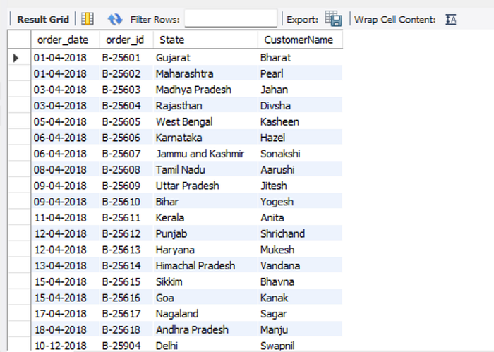
Query 5: Display the details (in terms of “order_date”, “order_id”, “State”, and “CustomerName”) for the first order in each state. Order the result by “order_id”.

In this case, I used ROW_NUMBER() function to assign the number for each order based on states and finally set the filter to only show the result for the first order for each state.

According to the result, Delhi is the last state where this Indian e-commerce website established its footprint. However, the profit generated from Delhi state is much higher than that from Gujarat state. Hence, we may conclude that the customers from Delhi truly have higher purchasing power. 😎
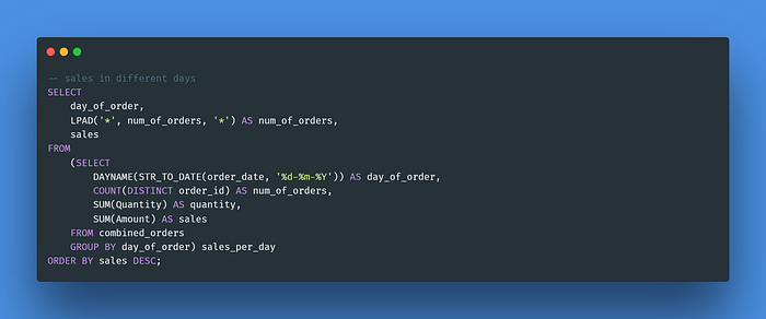
Query 6: Determine the number of orders (in the form of a histogram) and sales for different days of the week.

To return the weekday name for the “order_date”, we may use the DAYNAME() function. The next step is to pass the value returned by the COUNT DISTINCT function as an argument to the LPAD() function to control the number of * characters to return for each day.

The result of this query matches our expectation, whereby we could see that the highest sales happened on Sunday. However, if we are solely looking at the number of orders is the highest on Monday. This may happen because the customers selected the items they want to order on Sunday, and placed their orders on Monday.
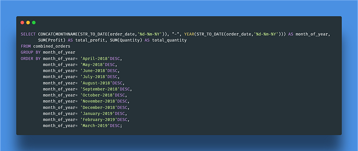
Query 7: Check the monthly profitability and monthly quantity sold to see if there are patterns in the dataset.

I used the MONTHNAME() and YEAR() functions to extract the month and year from the “order_date” after changing the “order_date” from string to date format using the STR_TO_DATE() function. You may note that I used CONCAT() function too. This is because I want to add a dash between the extractions. After that, I grouped the profit and quantity sold by the month using the GROUP BY clause and order the result based on the month in ascending order.

Losses occurred from April 2018 to September 2018. Luckily, there was a high profit from October 2018 onwards, followed along with an increase in the quantity sold (although it fluctuates). The total profit was able to cover all the losses it suffered previously. Besides, it also indicates that consumers started to shift toward online shopping.
However, a high number of products sold does not guarantee a high profit because the highest loss occurred in June 2018, but the quantity sold was the lowest in July 2018.
Query 8: Determine the number of times that salespeople hit or failed to hit the sales target for each category.

A new view called “sales_by_category” is created by grouping the “Category” and “Amount” by the “order_date”. Please note that the “order_date” was converted to the format that matches the date format in the table of “sales_target”.
Then, I created a new view called “sales_vs_target” by joining the “sales_by_category” with the “sales_target”. In this new view, the sales amount is compared with the sales target to return the result of either “Hit” or “Fail” using the CASE statement.
Finally, I extracted the number of times that the salespeople achieved or failed to achieve the target by performing inner join on two subqueries.

According to the result, the salespeople mostly failed to achieve the target for furniture and clothing target. It is needed to review the target to determine if it is achievable. Otherwise, more training would be required for the salespeople who are involved in promoting the furniture and clothing.
Query 9: Find the total sales, total profit, and total quantity sold for each category and sub-category. Return the maximum cost and maximum price for each sub-category too.

To find the total for quantity, profit, and amount, I used the SUM() function and stored the result in a new view called “order_details_by_total”.
After that, we need to find the cost of the product and the price of the product. The cost of the product is obtained by deducting the profit from the amount and dividing the result by the quantities sold, while the price of the product is obtained by dividing the amount by the quantities sold. To find the maximum cost and price, I used the MAX() function and stored the result in a new view called “order_details_by_unit”.
The final result is obtained by simply performing an inner join on the “order_details_by_total” and “order_details_by_unit” views.

All types of clothing made a profit. The top 3 best-selling sub-categories are under the category of clothing, and they are saree, handkerchief, and stole. The sellers can provide products that are complementary to these top 3 best-selling products to boost sales as there is a high chance that customers buy clothing products in pairs. For example, leggings and insoles.
On the other hand, the sellers should avoid selling electronic games and focus more on selling printers and accessories because electronic games led to losses although the quantity of electronic games is higher than that of printers and accessories.
This marks the end of my SQL project on the e-commerce dataset. Hope this article can shed some light on how to use SQL to perform data analysis on real-world datasets. Happy learning.😁
